

What nearest neighbor search actually does
The naive approach is called exact or brute-force nearest neighbor search — sometimes written exhaustive kNN search: compare the query vector against every single vector in your index, sort by distance, return the top results. It’s perfectly accurate and completely impractical. With ten million products at 1,024 dimensions, every query means ten billion multiply-add operations. You’d measure response times in seconds.
So real systems use approximate nearest neighbor search instead. The word “approximate” is doing enormous work here: these algorithms deliberately skip most of the dataset, accepting that they’ll occasionally miss a true nearest neighbor in exchange for being hundreds or thousands of times faster. Get 95–99% of the right answers in 5 milliseconds instead of 100% in 3 seconds — for product search, that’s not a hard call.
ANN, kNN, or vector similarity search? The same thing, four names
Before going further, a terminology detour that saves real confusion during vendor evaluations, because the industry never agreed on one name.
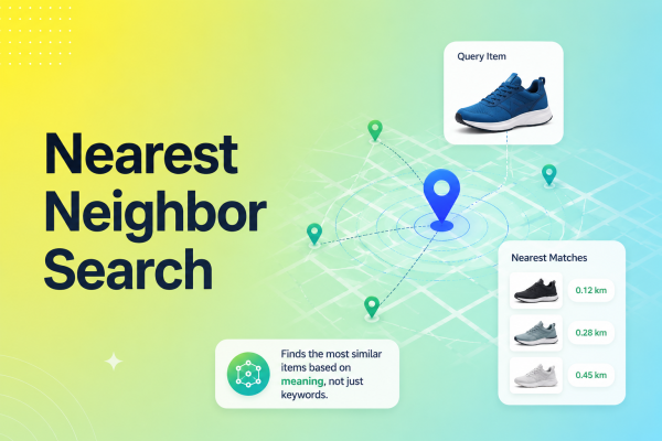
Nearest neighbor search is the general problem: find the items closest to a query item by distance.
kNN search — k-nearest neighbor search — is the precise version: return exactly the k closest items, checked against every candidate. Elasticsearch and OpenSearch both ship features literally named “kNN search,” which is why the abbreviation shows up constantly in documentation. Confusingly, their kNN implementations are usually approximate, not exhaustive.
ANN search — approximate nearest neighbor search — is the fast, slightly-imperfect version described throughout this guide. When a vendor advertises ANN search, they mean they’ve traded a small amount of recall for a very large amount of speed.
Vector similarity search is the marketing-friendly name favored by vector database vendors like Pinecone and Milvus. Mechanically it’s the same operation: embed, compare by distance, return the closest.
One more distinction worth holding onto: kNN classification, the classic machine-learning algorithm that labels a data point by polling its neighbors, is a different thing that shares the name. In an ecommerce context, kNN almost always means retrieval, not classification.
The practical takeaway when comparing platforms: ask which index structure sits underneath and whether results are exact or approximate. A vendor saying “vector similarity search” and a vendor saying “ANN search” may be running identical HNSW graphs — the label tells you about their marketing, not their engineering.
AI Search Grader by bCloud AI
Grade your ecommerce search in 10 quick questions
31% of ecommerce searches return zero results — and most shoppers who hit a dead end leave for a competitor. How does your store's search stack up?
Answer 10 short questions and get your AI search score, plus a personalized report to fix the gaps. Free, takes about 2 minutes.
No signup needed to take the quiz.
Understanding intent…
Scoring your answers across relevance, AI, experience, and insights.
Your AI search score is ready
Tell us where to send your personalized report. You'll see your score and recommendations right away.
Your score by pillar
Personalized recommendations
Fix the gaps in weeks, not quarters
bCloud AI replaces keyword-only search with hybrid AI retrieval — sub-200ms responses, 99.99% uptime, and conversion lifts of up to 40% across 50+ implementations.
2. How HNSW works — the algorithm you’re probably using
The dominant approach to approximate nearest neighbor search is HNSW, or Hierarchical Navigable Small World graphs, introduced in the 2016 paper by Malkov and Yashunin. If you use Pinecone, Qdrant, Weaviate, Elasticsearch, pgvector, or almost anything else, you’re running HNSW or a variant.
The intuition is a road network. Imagine finding an address across the country. You don’t check every street — you take the interstate to the right region, then a highway to the right city, then local roads to the block. HNSW builds exactly that structure over your vectors: multiple layers, where the top layer has very few nodes connected by long-range links, and each layer down gets denser with shorter links.
A query enters at the top layer and greedily walks toward vectors closer to it. When it can’t improve at that layer, it drops down and continues with finer-grained links. By the bottom layer it’s in the right neighborhood and only needs to examine a small local cluster. That’s how nearest neighbor search over millions of vectors finishes in single-digit milliseconds.
Two parameters control the trade-off. M sets how many links each node keeps — higher means better recall and more memory. efConstruction controls how thoroughly the graph is built, and efSearch controls how widely each query explores. Raising efSearch improves accuracy and costs latency, and it’s tunable per query, which is genuinely useful.
3. The alternatives to HNSW and when they matter
HNSW dominates, but it isn’t the only approach to approximate nearest neighbor search, and the alternatives solve real problems.
IVF (Inverted File Index) partitions the vector space into clusters, then searches only the clusters nearest your query. It uses far less memory than HNSW and builds faster, but recall is generally lower and it needs training on a representative sample. IVF shines at very large scale where HNSW’s memory appetite becomes the binding constraint.
Product Quantization (PQ) compresses vectors by splitting them into chunks and replacing each with a small code. It slashes memory dramatically — often 10 to 50 times — at some accuracy cost. Frequently combined as IVF-PQ for billion-scale deployments.
Scalar and binary quantization reduce precision per dimension rather than restructuring vectors, cutting memory with modest recall loss. Binary quantization is aggressive but pairs well with a rescoring pass on full-precision vectors.
Flat (brute-force), offered as exact kNN search in most systems, is worth mentioning because it’s genuinely correct below roughly 100,000 vectors on modern hardware. Don’t add nearest neighbor search complexity you don’t need.
DiskANN and disk-backed indexes keep most vectors on SSD rather than RAM, trading some latency for a much cheaper cost profile at scale.
The practical guidance: start with HNSW, add quantization when memory becomes the constraint, and consider IVF-PQ or disk-backed indexes past a few hundred million vectors. Our vector database comparison covers which systems support which.
4. The recall-versus-latency trade-off you have to make
This is the concept most teams skip, and it causes most nearest neighbor search disappointments.
Recall@k measures what fraction of the true top-k nearest neighbors your approximate index actually returned. If exact search would return ten specific products and your index returns nine of them, recall@10 is 0.9. This is the accuracy dial.
Every approximate nearest neighbor search system lets you trade recall against latency. Turn efSearch up and recall climbs while queries slow. Turn it down and queries fly while quality quietly degrades. There’s no universally correct setting — it depends on how much a miss costs you.
Here’s the part worth internalizing: low recall doesn’t produce error messages. It produces slightly worse results that nobody notices. A shopper who should have seen the perfect product sees the third-best instead, doesn’t love it, and leaves. Nothing in your monitoring flags it.
So measure it deliberately. Build a ground-truth set by running exact brute-force nearest neighbor search on a sample of real queries, then compare your production index against it. Target recall@10 above 0.95 for ecommerce; below 0.90 you’re losing conversions invisibly. Then validate the business impact using the methodology in our guides to search relevance metrics and A/B testing ecommerce search.
5. Filtering is where nearest neighbor search gets hard
Pure similarity is the easy case. Real ecommerce queries almost always add constraints: in stock, under $100, size medium, ships to this region. Combining filters with approximate nearest neighbor search is genuinely difficult, and it’s where implementations diverge sharply.
Pre-filtering applies constraints first, then searches within the surviving subset. Accurate, but it can break the graph structure — if your filter eliminates 99% of vectors, HNSW’s carefully built connections no longer lead anywhere useful, and performance collapses.
Post-filtering searches first, then discards results failing the filter. Fast and preserves the index, but you can end up with too few results, or none, if the filter is restrictive. Requesting extra candidates helps but doesn’t fully solve it.
Filtered HNSW integrates constraints into graph traversal itself, skipping non-matching nodes during the walk. This is the sophisticated option and the reason some vector databases significantly outperform others on filtered workloads.
When you evaluate any nearest neighbor search implementation, test it with your actual filters applied. Unfiltered benchmarks are close to meaningless for ecommerce, where nearly every query carries constraints.
What happens to nearest neighbor search when products change
Most explanations treat the index as static. Ecommerce catalogs never are.
Products arrive, sell out, and get rewritten every hour. However, graph indexes were not designed for constant churn. Three effects follow, and each one costs you quietly.
Inserts are expensive.
Adding a vector means walking the graph to find its neighbours, then rewiring links. That costs far more than adding a row to a keyword index. Consequently bulk imports can slow queries while they run.
Deletes are usually fake.
Removing a node would break the paths through it. So most systems mark it deleted and skip it instead. Those tombstones accumulate, wasting memory and slowing traversal until a rebuild clears them.
Graph quality drifts.
A graph built for one catalog degrades as that catalog changes shape. Recall falls slowly and silently. Therefore periodic rebuilds matter more than most teams expect.
In short, ask any vendor two questions. How long does a full rebuild take at your vector count? And does indexing run on separate resources from queries? Our real-time indexing guide covers the update path in detail.
Distance metrics: the choice underneath everything
One detail that quietly determines whether nearest neighbor search works: how you define “close.” Three metrics dominate, and they are not interchangeable.
Cosine similarity measures the angle between two vectors, ignoring their magnitude. It’s the default for text embeddings because it asks “do these point the same direction in meaning space?” rather than “are they the same size?” — and length in an embedding often reflects nothing more interesting than how long the source text was.
Dot product accounts for both angle and magnitude. On normalized vectors it produces the same ranking as cosine similarity but computes faster, which is why many systems normalize at index time and then use dot product internally. On unnormalized vectors it behaves differently and can bias toward longer documents.
Euclidean distance measures straight-line distance between points. It’s the intuitive choice and works well for some image and audio embeddings, but for text it tends to underperform cosine similarity.
The critical rule: use the metric your embedding model was trained with. Most modern text models are trained for cosine similarity, and pairing them with Euclidean distance degrades nearest neighbor search quality in ways that are easy to miss because nothing errors out — results just get subtly worse. Check the model card before configuring the index.
What good nearest neighbor search looks like in production
Pulling the threads together, a healthy setup has a few recognizable properties. Recall is measured against a brute-force ground truth on real queries, not assumed. Parameters are tuned deliberately, with efSearch set from a recall target rather than left at a default nobody chose. Filtered performance is benchmarked with actual production filters applied, since unfiltered numbers flatter almost every system. Memory headroom is planned, because HNSW graphs consume considerably more than the raw vectors suggest once link structures are counted. And the distance metric matches the embedding model.
That’s a real amount of ongoing engineering, which is the honest argument for managed platforms: the index layer has to be right, but it rarely differentiates your business. Teams building it themselves should budget for tuning and monitoring as continuing work, not a one-time setup task — recall drifts as catalogs grow, and nobody gets an alert when it does.
A note on benchmarks you’ll read online
Published ANN search benchmarks deserve skepticism. Most measure a single dataset with uniform vector distributions, no filters, no concurrent writes, and a warm cache — conditions no production ecommerce store ever operates under. A system that tops a public leaderboard can perform middling on a real catalog where every query carries stock and price constraints and the index is being updated continuously.
Run your own benchmark instead, on a sample of your actual catalog, with your actual filters, under simultaneous indexing load. It takes a day and tells you more than any published comparison. Measure recall against brute-force ground truth, latency at p95 and p99 rather than the average, and memory consumption at your projected catalog size rather than today’s.
How this fits into your search stack
Nearest neighbor search is one layer in a larger pipeline. An embedding model turns products and queries into vectors (embedding models guide). The ANN index retrieves candidates fast — that’s this article. Fusion blends those with keyword results (what is hybrid search). A reranker orders the final list (search reranking). For the broader picture, see what is vector search and the AI ecommerce search guide.
If tuning HNSW parameters and measuring recall isn’t where you want your engineers, managed platforms handle the index layer entirely. bCloud AI’s AI search engine manages nearest neighbor search, filtering, fusion, and reranking as one service, so you get sub-200ms retrieval without owning the algorithm.
Common Nearest Neighbor Search Mistakes That Hurt Search Performance
Building a fast nearest neighbor search system is only half the challenge. Many ecommerce teams deploy vector search successfully but unknowingly introduce configuration mistakes that reduce search quality, increase infrastructure costs, or slow down query performance. Understanding these pitfalls helps maintain both relevance and scalability as your catalog grows.
1. Using the Wrong Embedding Model
The quality of nearest neighbor search begins with the embedding model. If your embeddings were trained for semantic similarity but are indexed using an incompatible distance metric, retrieval quality can decline significantly. Always verify which similarity metric your embedding model was designed to use before building the index.
2. Ignoring Catalog Growth
An ANN index that performs well with 100,000 products may require different tuning after the catalog expands to several million products. Parameters such as graph connectivity, search depth, and memory allocation should be reviewed periodically instead of remaining fixed after the initial deployment.
3. Measuring Only Query Latency
Fast responses do not automatically mean good search. Teams often celebrate sub-50 ms retrieval times while overlooking declining relevance. Track both latency and business metrics such as click-through rate, add-to-cart rate, and conversion rate alongside recall measurements to understand the real customer experience.
4. Forgetting About Incremental Updates
Modern ecommerce catalogs constantly change as products are added, removed, or updated. Delayed indexing creates stale search results where customers cannot discover newly launched products or continue seeing unavailable inventory. A production-ready search pipeline should support efficient incremental indexing without rebuilding the entire vector index.
5. Optimizing for Benchmarks Instead of Customers
Public ANN benchmarks are useful for comparing algorithms, but they rarely reflect production workloads. Real shoppers apply filters, use incomplete queries, search with synonyms, and expect relevant results instantly. Evaluate nearest neighbor search using real customer queries, actual catalog data, and production traffic patterns rather than relying solely on benchmark scores.
Frequently asked questions
What is nearest neighbor search?
Nearest neighbor search finds the items in a dataset closest to a query item, measured by distance. In vector retrieval, closest means most similar in meaning, using cosine similarity or Euclidean distance. It’s the retrieval step underneath semantic and vector search.
What is approximate nearest neighbor search?
Approximate nearest neighbor search deliberately trades a small amount of accuracy for enormous speed gains. Instead of comparing a query against every vector, it uses index structures like HNSW to examine only a small fraction, typically returning 95–99% of the true nearest neighbors in milliseconds.
How does HNSW work?
HNSW builds a multi-layer graph over your vectors, where upper layers have sparse long-range links and lower layers are dense with short links. Queries enter at the top, greedily navigate toward closer vectors, then descend layer by layer — like taking highways before local roads.
What is kNN search, and how is it different from ANN search?
kNN search (k-nearest neighbor search) returns the k closest items to a query. Strictly, exact kNN search compares against every candidate; ANN search (approximate nearest neighbor search) uses an index like HNSW to examine only a fraction, trading a little recall for enormous speed. Most production systems advertising kNN search are actually running ANN search underneath.
Is vector similarity search the same as nearest neighbor search?
Yes, mechanically. Vector similarity search is the name many vector database vendors use for the same operation: embed the query, compare by distance such as cosine similarity, and return the closest vectors. The differences between products are in index structure, filtering support, and scale, not in the underlying concept.
What is recall in nearest neighbor search?
Recall@k measures what fraction of the true top-k nearest neighbors your approximate index returned. Recall of 0.95 means it found 95% of the correct results. It’s the accuracy dial you trade against latency, and low recall degrades results silently without any error.
Should I use HNSW or IVF?
Use HNSW for most workloads — it offers the best recall-latency balance and is the default in nearly every vector database. Consider IVF or IVF-PQ when memory cost becomes the binding constraint at very large scale, since they use far less RAM with somewhat lower recall.
How do filters affect nearest neighbor search?
Filters make it substantially harder. Pre-filtering can break graph connectivity when it eliminates most vectors; post-filtering can return too few results. Filtered HNSW integrates constraints into traversal and performs best. Always benchmark with your real filters applied.
Skip the index tuning.
bCloud AI manages nearest neighbor search, filtering, fusion, and reranking as one service — sub-200ms retrieval, no HNSW parameters to babysit.
bcloud.ai